Introduction

This manual is a hands-on tutorial on how to make perfusion and diffusion maps using software developed at the Massachusetts General Hospital NMR Center and distributed on this CD-ROM.

Included on this CD ROM are example datasets that you can use to generate perfusion maps with the program makeperf and diffusion maps with the program dmap.

Requirements

If you are not comfortable with the commands cd, ls, mv, mkdir, cp, rm, and more, please consult a basic Unix manual before trying to follow this tutorial.

The software has been designed to run on Sun workstations with the Solaris environment and on Linux 2.0 or higher with the scripting language Perl 5.001 or higher installed.

The image data should be in raw format, i.e. the pixel data should be stored contiguously by row, then slice or timepoint. The following types are supported: floats, shorts, unsigned shorts, longs, unsigned longs, byte and unsigned byte. The raw data files should end with the extension .bfloat, .bshort, .bushort, .blong, .bulong, .bchar and .buchar respectively. Big endian data format (SGI Irix, IBM RS6000, SUN) is assumed by default. For every raw image dataset, you need a header file which contains the following entries: number of rows, number of columns, number of slices or timepoints, and byte swapping flag. For example, for a big endian data set containing images of dimension 128x128 pixels and 46 time points, the header file would contain:

128 128 46 0

Getting Started

The CD ROM contains the following directories: bin, examples, and docs. In the bin directory you will find two subdirectories, Solaris and Linux, which contain the executables for computing perfusion and ADC maps for either Solaris or Linux 2.0 respectively. The examples directory contains one subdirectory: Study_1,which contains the subdirectories Perfusion and Diffusion. Both these directories contain two subdirectories data, where the actual raw image datasets are located, and maps which contains the example maps that have already been processed and to which you can compare your own results.

NB: First copy the CD ROM data over to your own Solaris or Linux system, otherwise you won't be able to write out your own perfusion maps. Also copy the executables (either the Linux or Solaris version) to the /bin directory on your system and make sure you place this directory in your path.

If you are not sure how to change your paths, please contact the system administrator of your Solaris or Linux system.

Making Perfusion Maps

This section will show you how to generate perfusion maps of regional Cerebral Blood Flow (rCBF), regional Cerebral Blood Volume (rCBV) and Mean Transit Time (MTT). More information on MR perfusion imaging can be found here

First,

cd Study_1/Perfusion

In this directory create a sub-directory, which will later on contain the perfusion maps that you will generate. Name it e.g. 'my_maps'. To do this type:

mkdir my_maps

cd my_maps

This means that makeperf needs 4 parameters to generate the perfusion maps. The first parameter is the raw data filename and includes the path and prefix of your image dataset, e.g. /perf_tutorial/example/study_1/in_, assuming that your dataset contains 11 slices (as in the sample dataset):

(Sample raw dataset of 11 slices in bshort format)

in00.bshort
in01.bshort
in02.bshort
..
..
in10.bshort

The second parameter is the filename extension used to indicate what type of data is stored. For our example it would be bshort. The third parameter, # slices, simply states the number of slices in your study e.g. 11. The fourth parameter, # timepoints, is the number of timepoints that you collected in your study, e.g. 46. An optional fifth argument can be used to specify the number of digits following your file name prefix, for example for the above case it would be 2, the default. In this tutorial we will use the dataset with the prefix in of type bshort which contains 11 slices and 46 timepoints. In the my_maps directory, type the following command:

makeperf ../data/in bshort 11 46

You will then see a list of contributors to the software development and documentation. There is also a pointer to this documentation.

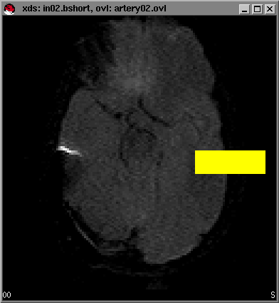
You will next see six windows pop up onto your screen, containing the first six slices from your dataset. These slices will be used to select the slice that contains the best visualization of the Middle Cerebral Artery (MCA) from which we will pick the Arterial Input Function (AIF). You can click on a window to make it active and press the + and - keys to circulate through all the timepoints in the dataset. In some instances you need to scale the signal intensities first in order to increase the image contrast (window and level settings). You can do this by moving the mousepointer over an area of the brain in the window and pressing the left mouse button, holding it down, dragging it to the right and down and releasing it. A yellow-highlighted area will appear that is referred to as a Region of Interest (ROI) and by pressing w the program will scale the image using the pixel data from the ROI you have drawn. Pressing C (shift-c) will delete the ROI from your window. An example is shown below using the window with slice #2 (in02.bshort).

Try experimenting with window and levelling by selecting different regions in the brain to give you the best image contrast. You can also change the window and level settings by pressing the middle mouse button while moving the mouse in the window. While scrolling through all the timepoints (+ and - keys) you will see the signal intensity decrease in the brain as the gadolinium (Gd) bolus is passing. This will help you to determine which slice contains the best visualization of the MCA since the signal drop in the major vessels is much greater than in the brain parenchyma itself. Sometimes you will have to wait a few seconds until the '*' sign in the right lower part of the windows disappears. This simply means that the system is loading the images into the main memory. The loading time will depend on the speed of your own computer system and will usually take less than 30 seconds.

For our example dataset, we have found that slice no.2 provides the best visualization of the MCA. Select this window by clicking on it. Next we will pick the arterial input function from the MCA by selecting points near the MCA that we want for our AIF. To do this: First type g from within the selected window (in this case the window for in02.bshort). A small timecourse window will pop-up and you will see the timecourse of the data graphically displayed as you move your mousepointer over the image of the brain slice in the window of in02.bshort.

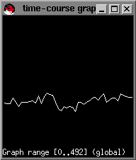
As soon as you enter the area of the MCA you will see a sharp drop in the signal intensity from the timecourse window. The decrease in the signal intensity indicates the pass of the bolus of contrast agent.

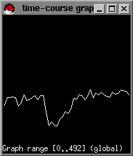
In this example, trace the right MCA territory, and when you see a sharp drop in signal intensity you click once on the left mouse button in the image window. Alternatively, you can type x to select the pixel below the mouse pointer. A yellow pixel will be displayed. If you want to erase a selected dot, move the mouse pointer over the spot and click it again. Alternatively, you can type c to erase the individual point pointed to by the mouse. To erase all the highlighted points type C. An example set of points that we have selected is shown below:

Each time you select a point, you can type s and the small window will show you a sample of the AIF, the average of your selected points, that is constructed from the data-points that you have selected so far.

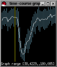
Typing g again will revert you to displaying the timecourse of the signal intensity under your mouse-pointer.
We can repeat this point and select process until a suitable AIF has been selected. Typically we have found a few pixels provided a good estimate of the AIF (the trade-off is higher SNR at the expense of dispersion). Once satisfied with the pixels you have selected for determining the AIF, you will need to save them for use in the SVD algorithm for determining rCBF and MTT. First make sure the window containing the MCA is active. Type O (not a zero but an uppercase o). A message will appear that an overlay file has been written. Then go to the window from which you typed the makeperf command (the command window), click on it to make it active. You will see a message prompting you to pick the AIF and reminding you to save the pixels you just picked. Type y followed by the [Enter] or [Return] key to confirm that this has been done:

Pick arterial input function.
Save ('O' in xds window.)
Enter y to continue: y

This step is needed to save the statistical information from the AIF that you selected for use by the program later on.

Go back to the command window and you will be prompted for the prefix of your input files:

Enter the prefix of your input files:
(e.g. 'in' for in00.bshort .. in10.bshort files)
Default: ../data/in

In this example, we can use the default value ../data/in, and you can just hit [Return].

Next you will be asked for the file type:

Enter the file type (e.g. bshort, bfloat, etc):
Default: bshort

Our example dataset is of type bshort, the default value, so again just hit [Return].

The next prompt will ask you for the number of slices:

Enter number of slices (default: 11)

In our example this is 11, so you can again just hit [Return].

Now you should enter a tag for the output files; this will be the prefix common to all of the processed images. In this tutorial we enter the name my_example

Enter a tag for the output files
my_example [Return]

You will next be prompted for the number of baseline images. This is the number of images before the sharp decrease in signal intensity. You can find this out by moving the mouse cursor to the last point on the time course graph before the signal drop and pressing the left mouse button.; the image number should appear in the bottom-left corner of the image window (in02.bshort window shown in lower left figure):

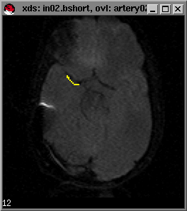
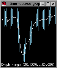
In this example, there are 12 baseline images or timepoints:

Enter number of baseline images
12 [Return]

You will now be asked to enter the last image to use for the computation of the perfusion maps:

This is the first image after the drop in signal intensity has recovered but before recirculation. The best way to select this is by drawing a larger ROI (as you did in adjusting the contrast in the image, previously), over a section of the brain parenchyma, not containing large vessels, or ventricles. Draw the ROI, type s and you can now select the last point in the graph after the sharp signal decrease but before recirculation. Again by hitting the mouse button in the timecourse window, the image number will appear in the bottom-left corner.

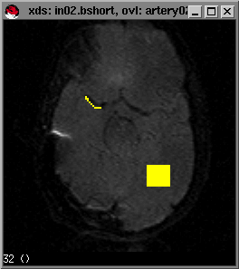
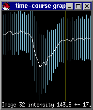
We typically want to integrate to the end of curve to avoid signal truncation unless the signal is too noisy at the end. In this case the last timepoint is 45 (since we count from 0).

Enter last image to use for CBF and MTT:
45 [Return]

Next you'll be asked to enter the number of the slice which contained the artery.

This is referring to the slice you used to select the Arterial Input Function from; it should be displayed along the top frame of the window. In the example, it is slice number two. So you just type 2 [Return].

From which slice is the artery?
Default: 00
2 [Return]

You will then be asked to confirm which file the AIF was selected from. In our example, we selected the AIF from in02.bshort. If the default is wrong (which can happen in the case of more than one AIF), we can override its value, but in this case we will type in the filename, although we could have just pressed [Return].

From which file is the artery?
Default: ../data/in02.bshort
../data/in02.bshort [Return]

You will then be prompted for the overlay name for which the AIF has been saved. makeperf by default saves the overlay files as artery[slice number].ovl. The .ovl was saved in the current working directory when you pressed O in the xds window. Since makeperf assumes the .ovl file will be in the same directory as the data, usually the case, we need to override the default:

What is the AIF overlay name (.ovl)?
Default: ../data/artery02.ovl
artery02.ovl [Return]

The same will hold true for the artery statistics file that will be computed from the .ovl file each time the program is run. makeperf always names the artery statistics file as artstats[slice number] and places it in your current working directory. So, in the example, you enter artstats02 [Return].

What will you call the artery statistics file?
Default: ../data/artstats02
artstats02 [Return]

Next you'll be prompted for the values to assign for TR, TE, and noise threshold. These values are determined by your MR imaging sequence . Use the default values only if they correspond to the values you used for TR, and TE. The noise threshold is the value that masks out the most noise while keeping the most parenchyma. Since we used the default values for our sample data, the default values will be used:

Enter TR (e.g. 1.5 for SE, 1.499 for GE):
Default: 1.5
1.5 [Return]

Enter TE (e.g. 0.075 for SE, 0.050 for GE):
Default: 0.075
0.075 [Return]

Enter noise threshold (e.g. 0.4 for SE, 0.25 for GE):
Default: 0.4
0.4 [Return]

Aberrant images to exclude (e.g. 7,17-20,29):
Default: none

Usually you don't need to exclude any images, so we leave it the default, none and just hit [Return]

The last step is selecting which kind of perfusion maps you want to be constructed next to the standard rCBF,rCBV and MTT maps. Just type the letter corresponding to the option you want, e.g. T if you also want Time To Peak maps.

Special map options: If you would like:
(R) Flow*R(t) (Residue function)
(c) uncorrected CBV
(p) K1 (CBV weighting) permeability
(j) K2 (T1 enhancement weighting)
(d) Average dR2 Mask
(A) Area
(a) Arrival Time
(Z) 1st moment / 0th moment
(T) Time to peak
(P) Peak value
(W) Area/Peak
(F) FWHM
(I) Initial slope
(D) Time to peak - Arrival time

Enter a string containing the letters corresponding to the maps you
want. Otherwise, just press return.

The naming conventions for the generated maps are respectively:

tag.R[slice number].bfloat
tag.sproUCBV.bfloat
tag.K1.bfloat
tag.K2.bfloat
tag.dR2.bfloat
tag.area.bfloat
tag.arrival.bfloat
tag.mom1_mom2.bfloat
tag.ttp.bfloat
tag.peak.bfloat
tag.ar_pk.bfloat
tag.fwhm.bfloat
tag.slope.bfloat
tag.relttp.bfloat

Residue function maps contain time course data, resulting in a separate data stack for each slice. tag refers to the tag variable you entered earlier, in this case, my_example. Otherwise all other data sets contain the results for all slices in one data stack.

For our example, we will not make maps in addition to rCBF,rUCBV, rCCBV and MTT maps and will just hit [Return]. You will now see:

Making perfmaps....please wait...

indicating that makeperf is generating the perfusion maps. This will take a few minutes (~30 minutes) depending on your CPU.

Once you see Done!, makeperf has finished and your perfusion maps will be in the my_maps directory, ready to be viewed with xds. Feel free to compare your results with the ones we have already provided in the maps directory.

makeperf generates files my_example.UCBV.bfloat, my_example.CBF.bfloat, my_example.MTT.bfloat and my_example.CCBV.bfloat and others you may have specified by the above parameters. MTT is computed using the central volume principle with values from UCBV and CBF. CCBV is the UCBV map corrected for changes in permeability in the blood brain barrier.

Making Diffusion Maps

First,

cd Study_1/Diffusion

In this directory create a sub-directory for the diffusion maps that you will generate. Name it my_maps. To do this type:

mkdir my_maps

cd my_maps

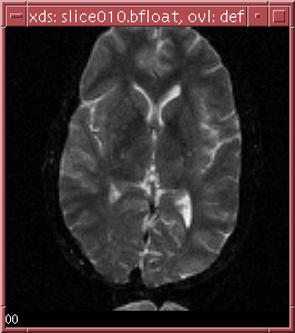
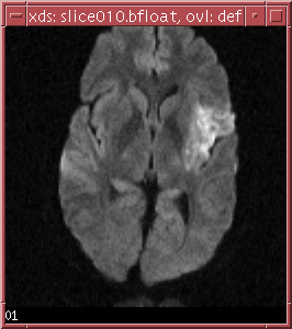
The b-values used are in the file specified by the -s option. The syntax of the script file is as follows:

image_number0 b_value0
image_number1 b_value1
...
image_numberN b_valueN

An optional argument is -n which specifies the threshold level to use to mask out non-brain can also be used.

To try dmap out on one slice 10, type the following command:

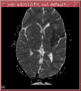
dmap -i ../data/slice010.bfloat -o adc010.flt -s dmap.script -n 8

An example shell script has been provided in ../maps/diffexec to process all 18 sample data slices and repack the output into a format readily viewable by xds. Copy over the diffexec and the dmap.script into your my_maps directory and run the script.

cp ../maps/diffexec diffexec
cp ../maps/dmap.script dmap.script
./diffexec

You are now ready to view your results using xds.

Viewing Results

To look at the actual perfusion maps that you generated with makeperf you use xds, an image viewing program.

From within the directory where your perfusion maps are located (in our example my_maps), you type

xds my_example.CBF.bfloat.

xds my_example.CBF.bfloat -z 2

For more advanced options press h from within the xds window and a list of advanced options of xds will be shown in the command window. By moving the mouse pointer over the images (e.g. the cbf map) the pixel values at the mouse-pointer will be displayed in the left-lower portion of the window. Notice that sometimes you will find negative pixelvalues in your CCBV,UCBV and MTT maps. This is due to not enough change in the raw data signal to reliably measure perfusion values at these pixels.

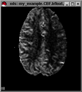
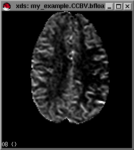
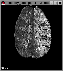
Example maps (from left to right) of rCBF,rCCBV and MTT respectively.